Introduction

Reinforcement Learning (RL) is a branch of Artificial Intelligence which consists in training or making learn an agent through reward to solve a problem, situation or act in an optimized manner within an environment.

The main difference with respect to supervised learning is that there is no ground truth or label. The training process is driven through reward. There also other differences such as the possible delay between an action and a the feedback or the influence of the agent in the environment, among others.

To clarify a little bit the situation, the following image can help:

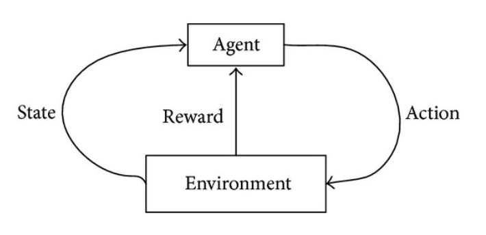
There are two main components of a RL optimization problem: the environment and the agent. The environment establishes the states or observations that the agent perceives and also the actions that the agent can take. For every action of the agent, there is a reward and a new observation.

Toy Example and Hard Coded Policy

To solve the problem, the agent must learn. However, for simples environments one can hard code the policy that the agent follows in order to succeed. In the MountainCar-V0, which is one of the simplest environments, one can devise a manual policy.

The environment is as follows:

The observation space is two dimensional Box of position and velocity, the car begins at (0, 0) and it has to go to 0.5, where the flag is placed. The action space, in the discrete case, is {0: Left, 1: Stop, 2: Right}

Hence, we can devise a policy that states that if the speed is positive go to the right, while if the speed is negative go to the left. Something like:

def policy(obs):
    position, velocity = obs

    if velocity > 0:
      action = actions['right']
    elif velocity < 0:
      action = actions['left']
    else:
      action = actions['left']

    return action

Then, we can hack the environment and make the car arrive at the objective. The full loop would be something like:

env = gym.make('MountainCar-v0')
env =  gym.wrappers.Monitor(env, './video/', force=True)
s = env.reset()
actions = {'left': 0, 'stop': 1, 'right': 2}

for i in range(1000):
    
    a = policy(s)
    obs, r, done, info = env.step(a)
    s = obs
    
    if done:
        break
env.close()

which would produce the following result:

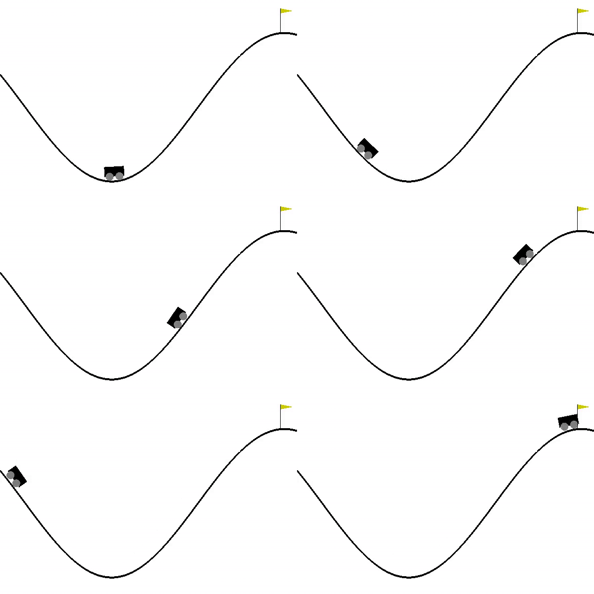
Obviously, this works here but it would be impossible to devise such hard coded policies for a complex environment. In the next section, Crossentropy method is used to be able to obtain a policy and update it by means of the rewards obtained.

Crossentropy method

The Crossentropy method is a importance sampling methodology that makes use of the crossentropy or Kullback-Leibler diveregence to drive a distribution close to another. It can either be used for estimation or optimization. From a simple view point, it involves an iterative process in which each step can be broken down into two pices:

Generate random sample from a distribution
Modify the parameters of the distribution

Algorithm

Here I will only detail the algorithm for a discrete space, for more details on the mathematical development and background you can check the guide from the original author.

$\mathbf{X}$ is a discrete valued space, $f$ is a distribution over $\mathbf{X}$ parametrized by probabilities $\mathbf{p}$ and $S$ is a performance function over $\mathbf{X}$. Also, we need a percentile value, $\rho$ which is going to be defined by hand. A crossentropy based optimization procedure would proceed as follows:

Initialize $f$ for $X$. Initialize time counter, $t$
Sample a sequence $\mathbf{X}_{1}$, …, $\mathbf{X}_{N}$ of points according to $f$.
Obtain performance values for each element of the sequence, $S_{1}$, …, $S_{N}$
Order them from smallest to biggest and let $\gamma_{t} = S_{(1-\rho)N}$ the $\rho$ quantile of the performance sequence.
Use the sample sample to update the probabilities $\mathbf{p}$ from the distribution $f$:

\[p_{t, j} = \frac{\sum_{i}^{N}I_{S(\mathbf{X}\_{i})\geq \gamma_{t}}I_{X_{ij} = 1}}{\sum_{i}^{N}I_{S(\mathbf{X}\_{i})\geq \gamma_{t}}}\]

Repeat 2-3 until convergence or meeting the stopping criterion.

In our case the $\mathbf{X}$ space is the action space, $f$ is the conditional probability distribution for every action being the environment in certain state s , $p(a|s)$ and the performance function is the reward function.

As we will see there is an important hypothesis in the scheme that we will be building and that will affect how the crossentropy procedure and its samplings are organized. The hypothesis is the Reward Hypothesis and says:

That all of what we mean by goals and purposes can be well thought of as maximization of the expected value of the cumulative sum of a received scalar signal (reward).

That is, instead of using the reward after every step, we will use the accumulated reward after an arbitrary number of steps to evaluate and modify the policy, $p(a|s)$.

Frozen Lake Example

In the frozen lake example, we are trying to go from the starting point S to the the other part of the frozen lake, our goal G, because we lost a frisbee (seriously, read the description of the game). Through the way there are walkable steps, F and holes H, where we can slip down an die (I guess that is what happens when you fall in a hole in a frozen lake because you lost your beloved frisbee, sigh). The possible actions for the agent are the movement directions: up, down, left or right. The observation space is the 4x4 (16 values) grid with every point defined as S, G, F or H. An example of grid is

  (Left)
SFFF
FHFH
FFFH
HFFG

There is the option to complicate the environment by making an 8x8 grid and making the surface of the lake slippery. The reward policy is 1 if the agent arrives to the other part of the frozen lake, and 0 otherwise.

To train the agent (the state-action table) which contains the conditional probabilities $p(a|s)$, we follow the Crossentropy algorithm. As state in the previous paragraph, we have 4 actions and 16 states, hence our decision matrix is 16 by 4.

The first step is to initialize the matrix, which would correspond to step 1. in the pseudo code of the crossentropy method.

import gym
import numpy as np

env = gym.make('FrozenLake-v0').env
policy = np.ones((env.observation_space.n, env.action_space.n))/env.action_space.n

In the next code piece all the rest of the steps are detailed:

for i in range(total_steps):
    
    # sample sessions according to p(a|s), step 2 in algorithm
    sessions = [generate_session(env, policy, steps_session) for j in range(n_sessions)]
    
    actions, states, rewards = zip(*sessions)
    
    # order the results from the samples and select best ones 
    # according to a percentile. step 3
    elite_states, elite_actions = select_elite(states, actions, rewards, percentile)
    
    # update policy. step 4
    new_policy = update_policy(elite_actions, elite_states)
    
    policy = learning_rate*new_policy + (1-learning_rate)*policy

In the second step, we sample the sessions and obtain the trajectories and rewards of each sequence, where the sampling is done through the current policy$

def generate_session(env, policy, t_max=10000):
    
    actions = []
    states = []
    reward = 0
    
    s = env.reset()
    for i in range(t_max):
        
        a = np.random.choice(range(env.action_space.n), p=policy[s, :])
        new_s, r, done, info  = env.step(a)
        
        actions.append(a)
        states.append(s)
        reward += r
        s = new_s
        
        if done:
            break
            
    return actions, states, reward

After this step, all the actions and states are collected as well as the reward obtained for each session. Remember the reward hypothesis and how we are collecting a reward for the whole session.

Now, we select the elite sessions, and their associated states and actions, throught the rewards obtaine. This corresponds to step 3:

def select_elite(states, actions, rewards, percentile=50):
    
    threshold = np.percentile(rewards, percentile)
    elite_states = sum([state for reward, state in zip( rewards, states) if reward > threshold], [])
    elite_actions = sum([action for reward, action in zip( rewards, actions) if reward > threshold], [])
    return elite_states, elite_actions

and finally we update the policy (Step 4) with the elite sessions data:

def update_policy(actions, states):
    
    policy_mat = np.zeros((env.observation_space.n, env.action_space.n))
    for i, j in zip(actions, states):
        policy_mat[j, i] +=1
    idx_not_visited = np.argwhere(policy_mat.sum(axis=1) == 0)
    policy_mat[idx_not_visited, :] = 1/env.action_space.n
    policy_mat = policy_mat/policy_mat.sum(axis=1)[:, np.newaxis]
    return policy_mat

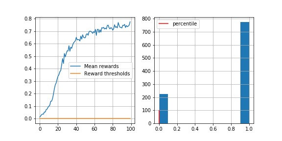
If we run this, we can check that the mean reward per session grows (reward threshold for a funtioning agent is at 0.78, env.spec.reward_threshold).

After training the agent, we can test it by running it once thorugh an environment. This is an example of a run:

Multiperceptron as posterior distribution

In the previous example, we have employed a matrix as a posterior distribution $p(a|s)$. That is, when we were on a specific state we sample the next action by using the posterior, which in our case was a table of dims $[S, A]$ where S was the number of states and A the numbers of actions. We updated this distribution by importance sampling on a group of sessions produced using the distribution but on the previous step.

The problem is that this method, using a tabular posterior distribution, can only work with discrete spaces. If we are in a continuous environment we have, at first hand, two simple solutions, one simpler than the other. First, to discretize the environment. The second is to use a construct that can handle a continuous distribution.

We will work on the second case using a Multi Layer Prerceptron (MLP) as posterior, for continuous environment observations and discrete actions. As environment we will work on the Lunar Lander.

Environment

The Lunar Lander is an environment where you must land a space shuttle on a rocky terrain.

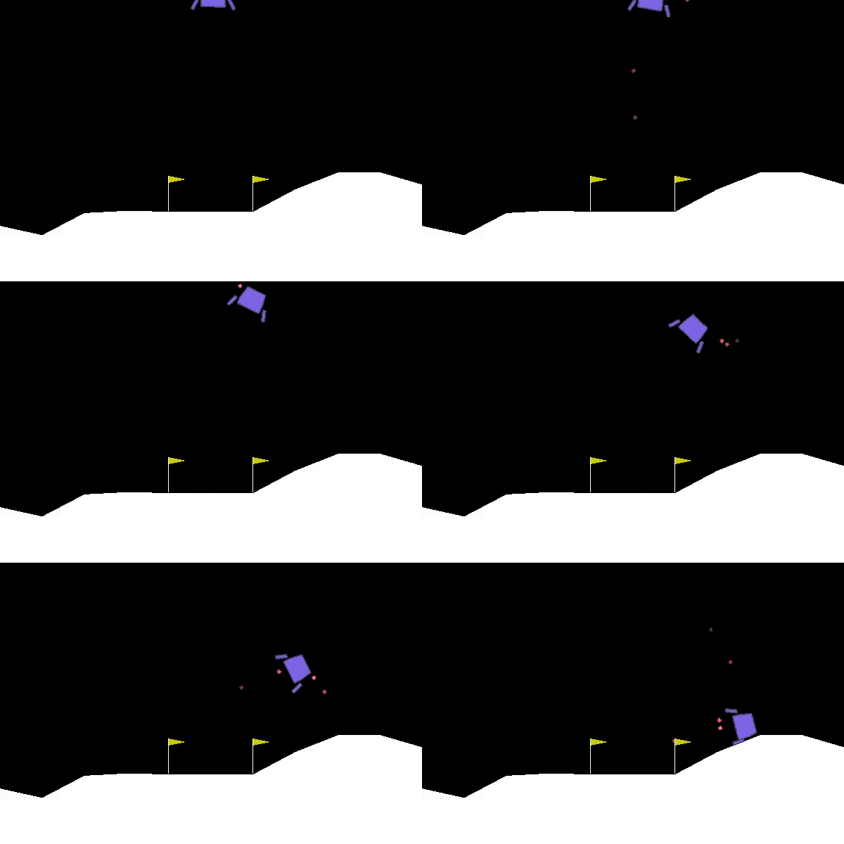
We will work with the discrete case. The action space consists in 4 actions: do nothing, move left, move right and sustain. The pad always begin at (0, 0) in the upper middle of the screen. The obervation space is a conitnuous vector of dimension 8, $\mathbf{x} \in \Bbb{R}^{8}$.

The reward scheme is more varied than in previous environments visited:

Moving towards the landing zone and zero speed is in the range of 100-140 points
If the shuttle moves aways from the landing zone it begins to lose points
If it crashes it receives -100, if it manages to land, receives 100
Landing outside landing zone is allowed, however, landing inside it carries a plus of 200 points.

Fuel is infinite.

MLP

There are only two things that change with respect our frozen lake procedure, since we are still using crossentropy:

The prediction of the action comes not from the posterior table, but from the MLP
Instead of updating the table with the rate of actions and the related states, we will train the MLP with the elite actions and states.

That is, we have no update_policy function, but a mlp.fit_partial(elite_states, elite_actions). Also, the prediction of an action from a environemnt observation is not a = np.random.choice(range(env.action_space.n), p=policy[s, :]) but

probs = agent.predict_proba(s.reshape(1, -1)).squeeze()
a = np.random.choice(range(n_actions), size=None, p=probs)

as can be seen, the MLP is used for building the logit distribution of actions.

The session generation will be now as:

def generate_session(env, agent, t_max=1000):

    states, actions = [], []
    total_reward = 0

    s = env.reset()

    for t in range(t_max):
        
        probs = agent.predict_proba(s.reshape(1, -1)).squeeze()#<YOUR CODE>
        a = np.random.choice(range(n_actions), size=None, p=probs) #<YOUR CODE>
        new_s, r, done, info = env.step(a)

        states.append(s)
        actions.append(a)
        total_reward += r

        s = new_s
        if done:
            break
    return actions, states, total_reward

Note that we only change the way how the actions probabilities are built. And the full training:

percentile = 50
steps_session = 2000
n_sessions = 100
total_steps = 100

env = gym.make('LunarLander-v2').env
mlp = neural_network.MLPClassifier((128, 64), activation='tanh', learning_rate_init=0.001)
mlp.partial_fit([env.reset()]*n_actions, range(n_actions), range(n_actions))
log = []

for i in range(total_steps):
    
    sessions = Parallel(n_jobs=cpu_count())(delayed(generate_session)(env, mlp, steps_session) for j in range(n_sessions))
    actions, states, rewards = zip(*sessions)
    
    elite_states, elite_actions = select_elite(states, actions, rewards, percentile)
    mlp.partial_fit(elite_states, np.asarray(elite_actions).reshape(-1, 1))
    
    show_progress(rewards, log, percentile, reward_range=[-500, 400])

Which should arrives or surpass the reward threshold of 200 stablished for this environment.

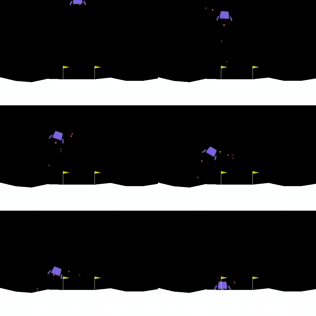
An example of a trainer agent:

Conclusion

In this post we have learnt about the components of a Reinforcement Learning method: agent and environment. And its associated actionables and observables, actions and states, respectively. We have also learned about the crossentropy method, which is an importance sampling procedure, and how it can be useful to train an agent. Finally, we have also learnt to substitute the discrete posterior distribution table for an object that can handle continuous entries, the Multi Layer Perceptron. With this we have been able to train the Lunar Lander which has continuous variables for the observations.

In the next post, we will learn about value and state functions and how we can improve the crossentropy method for training an agent.

All the code used in this post can be found at the github site of this web page under the folder code

RL Part I: First steps in reinforcement learning with OpenAI Gym

OpenAI Gym Environment, hand made policies and Crossentropy method.